【scikit-learn】データセット自作用ツールまとめ – 概要、使い方を解説

Pythonの機械学習ライブラリであるscikit-learnには、実験用のデータセットを自作するためのツール（関数）が用意されています。

これを利用することで行いたい機械学習手法の実験に合わせたデータセットの自作が可能です。

この記事では、scikit-learnのデータセット自作用ツールの概要と使い方を解説します。

データセット自作用ツールの概要

まずはデータセット自作用ツールの概要を簡単に説明します。

データセット自作用ツールの意義

scikit-learnには実験用のデータセットが付属していますが、これらはデータ件数や次元数などが定まっているため、使用する上で不都合が生じる場合もあります。

データセット自作用ツールを使えばデータ件数や次元数を自由に設定して実験用のデータセットを一から自作できるため、そのような心配はなくなります。

データセット自作用ツールの使い方

データセット自作用ツールはsklearn.datasetsクラスからインポートして利用します。

インポートしたデータセット自作用ツール（関数）にパラメータを設定することで、入力データと正解データを得ることができます。

設定できるパラメータはツールによって異なるため、パラメータについての説明は後述します。

データセット自作用ツール一覧

scikit-learnのデータセット自作用ツールは全部で20個です。

各ツールについての基本的な情報とその使い方を解説します。

make_blobs()

クラスタ数や標準偏差を指定して多クラスのデータセットを生成します。

• 用途：分類、クラスタリング
• ドキュメント：sklearn.datasets.make_blobs

以下にmake_blobs()の使用例を示します。

from sklearn.datasets import make_blobs
import matplotlib.pyplot as plt

if __name__ == "__main__":

    n_samples = 500            # データ件数
    n_features = 2             # データ次元数
    centers = 3                # クラスタ数
    cluster_std = 1.0          # クラスタの標準偏差
    center_box = (-10.0, 10.0) # 各クラスタ中心の境界ボックス
    shuffle = True             # データセットをシャッフルする
    random_state = 1           # 乱数生成用のシード

    # make_blobs()を用いてデータを作成
    x, y = make_blobs(n_samples=n_samples, n_features=n_features, centers=centers, cluster_std=cluster_std, center_box=center_box, shuffle=shuffle, random_state=random_state)

    # 生成されたデータをプロットする
    classes = list(set(y))
    for i in classes:
        dots = x[ y==i ]
        plt.scatter(dots[:,0], dots[:,1])
    plt.title('make_blobs')
    plt.show()

このプログラムを実行すると以下の出力結果が得られます。

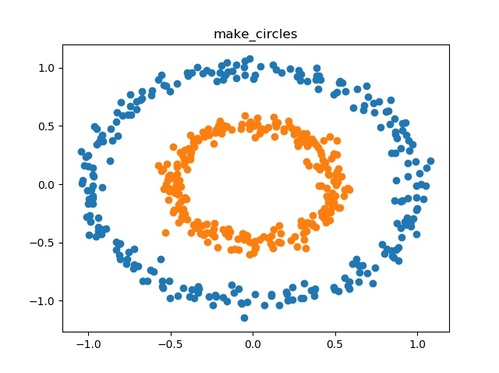
make_circles()

二次元の小さな円を含む大きな円を作成します。

• 用途：分類、クラスタリング
• ドキュメント：sklearn.datasets.make_circles

以下にmake_circles()の使用例を示します。

from sklearn.datasets import make_circles
import matplotlib.pyplot as plt

if __name__ == "__main__":

    n_samples = 500   # データ件数
    factor = 0.5      # 内側と外側の円の間のスケール係数
    noise = 0.05      # ノイズの標準偏差
    shuffle = True    # データセットをシャッフルする
    random_state = 1  # 乱数生成用のシード

    # make_circles()を用いてデータを生成する
    x, y = make_circles(n_samples=n_samples, factor=factor, noise=noise, shuffle=shuffle, random_state=random_state)

    # 生成されたデータをプロットする
    classes = list(set(y))
    for i in classes:
        dots = x[ y==i ]
        plt.scatter(dots[:,0], dots[:,1])
    plt.title('make_circles')
    plt.show()

このプログラムを実行すると以下の出力結果が得られます。

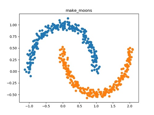
make_moons()

二つの入り組んだ半円を作成します。

• 用途：分類、クラスタリング
• ドキュメント：sklearn.datasets.make_moons

以下にmake_moons()の使用例を示します。

from sklearn.datasets import make_moons
import matplotlib.pyplot as plt

if __name__ == "__main__":

    n_samples = 500   # データ件数
    noise = 0.05      # ノイズの標準偏差
    shuffle = True    # データセットをシャッフルする
    random_state = 1  # 乱数生成用のシード

    # make_moons()を用いてデータを生成する
    x, y = make_moons(n_samples=n_samples, noise=noise, shuffle=shuffle, random_state=random_state)

    # 生成されたデータをプロットする
    classes = list(set(y))
    for i in classes:
        dots = x[ y==i ]
        plt.scatter(dots[:,0], dots[:,1])
    plt.title('make_moons')
    plt.show()

このプログラムを実行すると以下の出力結果が得られます。

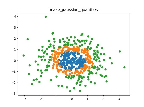
make_gaussian_quantiles()

等方性ガウス分布を生成し、分位によってサンプルにラベルを付けます。

• 用途：分類
• ドキュメント：sklearn.datasets.make_gaussian_quantiles

以下にmake_gaussian_quantiles()の使用例を示します。

from sklearn.datasets import make_gaussian_quantiles
import matplotlib.pyplot as plt

if __name__ == "__main__":

    n_samples = 500   # データ件数
    n_features = 2    # データ次元数
    n_classes = 3     # クラスの数
    mean = (0,0)      # 多次元正規分布の平均
    cov = 1.0         # 共分散行列の計算に使用
    shuffle = True    # データセットをシャッフルする
    random_state = 1  # 乱数生成用のシード

    # make_gaussian_quantiles()を用いてデータを生成する
    x, y = make_gaussian_quantiles(n_samples=n_samples, n_features=n_features, n_classes=n_classes, mean=mean, cov=cov, shuffle=shuffle, random_state=random_state)

    # 生成されたデータをプロットする
    classes = list(set(y))
    for i in classes:
        dots = x[ y==i ]
        plt.scatter(dots[:,0], dots[:,1])
    plt.title('make_gaussian_quantiles')
    plt.show()

このプログラムを実行すると以下の出力結果が得られます。

make_hastie_10_2()

ガウス関数によって生成された10個の特徴量を持つデータセットを作成します。なお、次数の指定は不可です。

• 用途：分類、クラスタリング
• ドキュメント：sklearn.datasets.make_hastie_10_2

以下にmake_hastie_10_2()の使用例を示します。

from sklearn.datasets import make_hastie_10_2

if __name__ == "__main__":

    n_samples = 50    # データ件数
    random_state = 1  # 乱数生成用のシード

    # make_hastie_10_2()を用いてデータを生成する
    x, y = make_hastie_10_2(n_samples=n_samples, random_state=random_state)

    # 生成されたデータを表示する
    print('x.shape : {}'.format(x.shape))
    print(x)
    print('y.shape : {}'.format(y.shape))
    print(y)

このプログラムを実行すると以下の出力結果が得られます。

x.shape : (50, 10)
[[ 1.62434536e+00 -6.11756414e-01 -5.28171752e-01 -1.07296862e+00
   8.65407629e-01 -2.30153870e+00  1.74481176e+00 -7.61206901e-01
   3.19039096e-01 -2.49370375e-01]
...
 [-1.05344713e-01  6.30195671e-01 -4.14846901e-01  4.51946037e-01
  -1.57915629e+00 -8.28627979e-01  5.28879746e-01 -2.23708651e+00
  -1.10771250e+00 -1.77183179e-02]]
y.shape : (50,)
[ 1.  1. -1. -1.  1. -1.  1. -1. -1. -1. -1. -1.  1. -1. -1.  1.  1.  1.
 -1.  1.  1. -1.  1.  1. -1.  1. -1.  1. -1. -1.  1.  1. -1.  1. -1. -1.
  1.  1. -1.  1.  1.  1. -1.  1.  1. -1. -1.  1.  1.  1.]

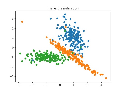
make_classification()

make_blobs()と同様に多クラスのデータセットを生成します。情報的価値のない特徴量などのノイズをデータセットに加えることも可能です。

• 用途：分類、クラスタリング
• ドキュメント：sklearn.datasets.make_classification

以下にmake_classification()の使用例を示します。

from sklearn.datasets import make_classification
import matplotlib.pyplot as plt

if __name__ == "__main__":

    n_samples = 500           # データ件数
    n_features = 2            # データ次元数
    n_informative = 2         # 情報価値のある特徴量の数
    n_redundant = 0           # 冗長な特徴量の数
    n_repeated = 0            # 複製する特徴量の数
    n_classes = 3             # クラスの数
    n_clusters_per_class = 1  # クラスごとのクラスタの数
    weights = None            # クラスごとのデータの割合
    flip_y = 0.01             # ランダムに交換されるデータの割合
    class_sep = 1.0           # ハイパーキューブサイズを乗算する係数
    hypercube = True          # クラスタをハイパーキューブの頂点に配置する
    shift = 0.0               # 指定した値だけ特徴量をシフトする
    scale = 1.0               # 指定した値で特徴量を乗算する
    shuffle = True            # データセットをシャッフルする
    random_state = 1          # 乱数生成用のシード

    # make_classification()を用いてデータを生成する
    x, y = make_classification(n_samples=n_samples, n_features=n_features, n_informative=n_informative, n_redundant=n_redundant, n_repeated=n_repeated, n_classes=n_classes, n_clusters_per_class=n_clusters_per_class, weights=weights, flip_y=flip_y, class_sep=class_sep, hypercube=hypercube, shift=shift, shuffle=shuffle, random_state=random_state)

    # 生成されたデータをプロットする
    classes = list(set(y))
    for i in classes:
        dots = x[ y==i ]
        plt.scatter(dots[:,0], dots[:,1])
    plt.title('make_classification')
    plt.show()

このプログラムを実行すると以下の出力結果が得られます。

make_multilabel_classification()

ランダムなマルチラベル分類問題を生成します。

• 用途：分類、クラスタリング
• ドキュメント：sklearn.datasets.make_multilabel_classification

以下にmake_multilabel_classification()の使用例を示します。

from sklearn.datasets import make_multilabel_classification

if __name__ == "__main__":

    n_samples = 100               # データ件数
    n_features = 10               # データ次元数
    n_classes = 5                 # クラスの数
    n_labels = 2                  # インスタンスごとのラベルの平均
    length = 50                   # 特徴量の合計
    allow_unlabeled = True        # どのクラスにも属さないインスタンスの有無
    sparse = False                # Sparse Feature Matrixを返さない
    return_indicator = 'dense'    # 正解ラベルをバイナリーで表示
    return_distributions = False  # p_c、p_w_cを返さない
    random_state = 1              # 乱数生成用のシード

    # make_multilabel_classification()を用いてデータを生成する
    x, y = make_multilabel_classification(n_samples=n_samples, n_features=n_features, n_classes=n_classes, n_labels=n_labels, length=length, allow_unlabeled=allow_unlabeled, sparse=sparse, return_indicator=return_indicator, return_distributions=return_distributions, random_state=random_state)

    # 生成されたデータを表示する
    print('x.shape : {}'.format(x.shape))
    print(x)
    print('y.shape : {}'.format(y.shape))
    print(y)

このプログラムを実行すると以下の出力結果が得られます。

x.shape : (100, 10)
[[ 6.  5.  7.  2.  5.  2.  5. 10.  5.  4.]
 [ 5.  9.  1.  6.  0.  0.  5.  5.  8.  7.]
...
 [ 4.  4. 10.  8. 10.  1.  2. 10.  3.  0.]
 [ 3.  4.  8.  8.  1.  3.  3. 13.  9.  3.]]
y.shape : (100, 5)
[[0 0 0 0 0]
 [0 1 0 0 0]
...
 [1 0 0 0 0]
 [1 1 0 0 0]]

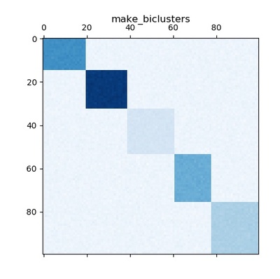
make_biclusters()

バイクラスタリング用の一定のブロック対角構造を持つ配列を生成します。

• 用途：バイクラスタリング
• ドキュメント：sklearn.datasets.make_biclusters

以下にmake_biclusters()の使用例を示します。

from sklearn.datasets import make_biclusters
import matplotlib.pyplot as plt

if __name__ == "__main__":

    shape = (100, 100)  # 出力の形状
    n_clusters = 5      # クラスタ数
    noise = 1           # ノイズの標準偏差
    minval = 10         # バイクラスターの最小値
    maxval = 100        # バイクラスターの最大値
    shuffle = False     # データセットをシャッフルしない
    random_state = 1    # 乱数生成用のシード

    # make_biclusters()を用いてデータを生成する
    x, rows, cols = make_biclusters(shape=shape, n_clusters=n_clusters, noise=noise, minval=minval, maxval=maxval, shuffle=shuffle, random_state=random_state)

    # 生成されたデータをプロットする
    plt.matshow(x, cmap=plt.cm.Blues)
    plt.title("make_biclusters")
    plt.show()

このプログラムを実行すると以下の出力結果が得られます。

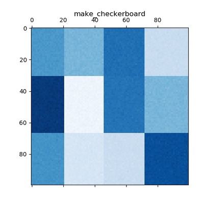
make_checkerboard()

バイクラスタリング用のブロックチェッカーボード構造を持つ配列を生成します。

• 用途：バイクラスタリング
• ドキュメント：sklearn.datasets.make_checkerboard

以下にmake_checkerboard()の使用例を示します。

from sklearn.datasets import make_checkerboard
import matplotlib.pyplot as plt

if __name__ == "__main__":

    shape = (100, 100)  # 出力の形状
    n_clusters = (3,4)  # クラスタ数
    noise = 1           # ノイズの標準偏差
    minval = 10         # バイクラスターの最小値
    maxval = 100        # バイクラスターの最大値
    shuffle = False     # データセットをシャッフルしない
    random_state = 1    # 乱数生成用のシード

    # make_checkerboard()を用いてデータを生成する
    x, rows, cols = make_checkerboard(shape=shape, n_clusters=n_clusters, noise=noise, minval=minval, maxval=maxval, shuffle=shuffle, random_state=random_state)

    # 生成されたデータをプロットする
    plt.matshow(x, cmap=plt.cm.Blues)
    plt.title("make_checkerboard")
    plt.show()

このプログラムを実行すると以下の出力結果が得られます。

make_regression()

ランダムな回帰問題を生成します。

• 用途：回帰
• ドキュメント：sklearn.datasets.make_regression

以下にmake_regression()の使用例を示します。

from sklearn.datasets import make_regression

if __name__ == "__main__":

    n_samples = 100        # データ件数
    n_features = 10        # データ次元数
    n_informative = 6      # 情報価値のある特徴量の数
    n_targets = 1          # 出力次元数
    bias = 0.0             # バイアス
    effective_rank = None  # 入力に単位分散を含む
    tail_strength = 0.5    # tailの相対的な重要性
    noise = 0.0            # ノイズの標準偏差
    shuffle = False        # データセットをシャッフルしない
    coef = False           # 線形モデルの係数を返さない
    random_state = 1       # 乱数生成用のシード

    # make_regression()を用いてデータを生成する
    x, y = make_regression(n_samples=n_samples, n_features=n_features, n_informative=n_informative, n_targets=n_targets, bias=bias, effective_rank=effective_rank, tail_strength=tail_strength, noise=noise, shuffle=shuffle, coef=coef, random_state=random_state)

    # 生成されたデータを表示する
    print('x.shape : {}'.format(x.shape))
    print(x)
    print('y.shape : {}'.format(y.shape))
    print(y)

このプログラムを実行すると以下の出力結果が得られます。

x.shape : (100, 10)
[[ 1.62434536e+00 -6.11756414e-01 -5.28171752e-01 -1.07296862e+00
   8.65407629e-01 -2.30153870e+00  1.74481176e+00 -7.61206901e-01
   3.19039096e-01 -2.49370375e-01]
...
 [ 1.60564992e-01 -1.20149976e-01  3.85602292e-01  7.18290736e-01
   1.29118890e+00 -1.16444148e-01 -2.27729800e+00 -6.96245395e-02
   3.53870427e-01 -1.86955017e-01]]
y.shape : (100,)
[-111.00477947  -76.42618232   95.41793893 -164.70718785   62.58454431
...
   46.81241123 -144.4124635  -156.16394589  -39.38189868  119.69071537]

make_sparse_uncorrelated()

非相関のスパースに基づくランダムな回帰問題を生成します。（最初の４つの特徴量のみ情報的価値を持ち、残りは情報的価値を持ちません。）

• 用途：回帰
• ドキュメント：sklearn.datasets.make_sparse_uncorrelated

以下にmake_sparse_uncorrelated()の使用例を示します。

from sklearn.datasets import make_sparse_uncorrelated

if __name__ == "__main__":

    n_samples = 100   # データ件数
    n_features = 10   # データ次元数
    random_state = 1  # 乱数生成用のシード

    # make_sparse_uncorrelated()を用いてデータを生成する
    x, y = make_sparse_uncorrelated(n_samples=n_samples, n_features=n_features, random_state=random_state)

    # 生成されたデータを表示する
    print('x.shape : {}'.format(x.shape))
    print(x)
    print('y.shape : {}'.format(y.shape))
    print(y)

このプログラムを実行すると以下の出力結果が得られます。

x.shape : (100, 10)
[[ 1.62434536e+00 -6.11756414e-01 -5.28171752e-01 -1.07296862e+00
   8.65407629e-01 -2.30153870e+00  1.74481176e+00 -7.61206901e-01
   3.19039096e-01 -2.49370375e-01]
...
 [ 1.60564992e-01 -1.20149976e-01  3.85602292e-01  7.18290736e-01
   1.29118890e+00 -1.16444148e-01 -2.27729800e+00 -6.96245395e-02
   3.53870427e-01 -1.86955017e-01]]
y.shape : (100,)
[  2.91339281  -3.86976605  -0.86011037   0.83295373  -4.5225354
...
  -2.31474361   3.90281713   5.35163114  -0.48105322  -1.5823179 ]

make_friedman1()

Friedman＃1回帰問題を生成します。（情報的価値を持つ特徴量は5つだけで、残りの特徴量は情報的価値を持ちません。）

• 用途：回帰
• ドキュメント：sklearn.datasets.make_friedman1

以下にmake_friedman1()の使用例を示します。

from sklearn.datasets import make_friedman1

if __name__ == "__main__":

    n_samples = 100   # データ件数
    n_features = 10   # データ次元数
    noise = 0.0       # ノイズの標準偏差
    random_state = 1  # 乱数生成用のシード

    # make_friedman1()を用いてデータを生成する
    x, y = make_friedman1(n_samples=n_samples, n_features=n_features, noise=noise, random_state=random_state)

    # 生成されたデータを表示する
    print('x.shape : {}'.format(x.shape))
    print(x)
    print('y.shape : {}'.format(y.shape))
    print(y)

このプログラムを実行すると以下の出力結果が得られます。

x.shape : (100, 10)
[[4.17022005e-01 7.20324493e-01 1.14374817e-04 3.02332573e-01
  1.46755891e-01 9.23385948e-02 1.86260211e-01 3.45560727e-01
  3.96767474e-01 5.38816734e-01]
...
 [8.12507304e-01 2.83801835e-01 5.27846796e-01 3.39416724e-01
  5.54667311e-01 9.74403469e-01 3.11702918e-01 6.68796606e-01
  3.25967207e-01 7.74477266e-01]]
y.shape : (100,)
[16.85220495 18.51319661 18.48797161 14.28170526 16.66632041  7.18940637
...
 15.29485529 20.08116211  7.46155257 12.8100486 ]

make_friedman2()

Friedman＃2回帰問題を生成します。（※特徴量の数は4つで固定です。）

• 用途：回帰
• ドキュメント：sklearn.datasets.make_friedman2

以下にmake_friedman2()の使用例を示します。

from sklearn.datasets import make_friedman2

if __name__ == "__main__":

    n_samples = 100   # データ件数
    noise = 0.0       # ノイズの標準偏差
    random_state = 1  # 乱数生成用のシード

    # make_friedman2()を用いてデータを生成する
    x, y = make_friedman2(n_samples=n_samples, noise=noise, random_state=random_state)

    # 生成されたデータを表示する
    print('x.shape : {}'.format(x.shape))
    print(x)
    print('y.shape : {}'.format(y.shape))
    print(y)

このプログラムを実行すると以下の出力結果が得られます。

x.shape : (100, 4)
[[4.17022005e+01 1.30240610e+03 1.14374817e-04 4.02332573e+00]
...
 [3.81016124e+01 1.35065337e+03 5.11141478e-01 6.40951805e+00]]
y.shape : (100,)
[  41.70246584   53.55222749  423.52599783   47.3689695   151.62674354
...
 1065.63674407  416.30072848  202.79642335  105.60691267  691.42545621]

make_friedman3()

Friedman＃3回帰問題を生成します。（※特徴量の数は4つで固定です。）

• 用途：回帰
• ドキュメント：sklearn.datasets.make_friedman3

以下にmake_friedman3()の使用例を示します。

from sklearn.datasets import make_friedman3

if __name__ == "__main__":

    n_samples = 100   # データ件数
    noise = 0.0       # ノイズの標準偏差
    random_state = 1  # 乱数生成用のシード

    # make_friedman3()を用いてデータを生成する
    x, y = make_friedman3(n_samples=n_samples, noise=noise, random_state=random_state)

    # 生成されたデータを表示する
    print('x.shape : {}'.format(x.shape))
    print(x)
    print('y.shape : {}'.format(y.shape))
    print(y)

このプログラムを実行すると以下の出力結果が得られます。

x.shape : (100, 4)
[[4.17022005e+01 1.30240610e+03 1.14374817e-04 4.02332573e+00]
...
 [3.81016124e+01 1.35065337e+03 5.11141478e-01 6.40951805e+00]]
y.shape : (100,)
[0.00356746 1.29320233 1.47697679 1.12451239 1.29197939 1.42226939
...
 1.51125299 1.54272043 1.28539207 1.51566251]

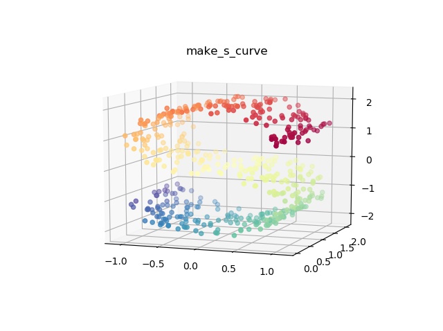
make_s_curve()

S字カーブを生成します。（※特徴量の数は固定）

• 用途：多様体学習
• ドキュメント：sklearn.datasets.make_s_curve

以下にmake_s_curve()の使用例を示します。

from sklearn.datasets import make_s_curve
from mpl_toolkits.mplot3d import Axes3D
import matplotlib.pyplot as plt

if __name__ == "__main__":

    n_samples = 500   # データ件数
    noise = 0.05      # ノイズの標準偏差
    random_state = 1  # 乱数生成用のシード

    # make_s_curve()を用いてデータを生成する
    x, color = make_s_curve(n_samples=n_samples, noise=noise, random_state=random_state)

    # 生成されたデータをプロットする
    fig = plt.figure()
    ax = fig.add_subplot(111, projection='3d')
    ax.scatter(x[:,0], x[:,1], x[:,2], c=color, cmap=plt.cm.Spectral)
    ax.view_init(10, -70)
    plt.title('make_s_curve')
    plt.show()

このプログラムを実行すると以下の出力結果が得られます。

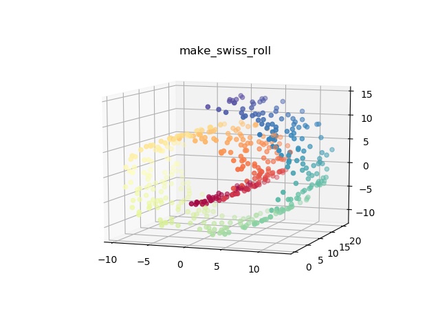
make_swiss_roll()

スイスロールを生成します。（※特徴量の数は固定）

• 用途：多様体学習
• ドキュメント：sklearn.datasets.make_swiss_roll

以下にmake_swiss_roll()の使用例を示します。

from sklearn.datasets import make_swiss_roll
from mpl_toolkits.mplot3d import Axes3D
import matplotlib.pyplot as plt

if __name__ == "__main__":

    n_samples = 500   # データ件数
    noise = 0.05      # ノイズの標準偏差
    random_state = 1  # 乱数生成用のシード

    # make_swiss_roll()を用いてデータを生成する
    x, color = make_swiss_roll(n_samples=n_samples, noise=noise, random_state=random_state)

    # 生成されたデータをプロットする
    fig = plt.figure()
    ax = fig.add_subplot(111, projection='3d')
    ax.scatter(x[:,0], x[:,1], x[:,2], c=color, cmap=plt.cm.Spectral)
    ax.view_init(10, -70)
    plt.title('make_swiss_roll')
    plt.show()

このプログラムを実行すると以下の出力結果が得られます。

make_low_rank_matrix()

ベル型の特異値を使用して、ほとんど低ランクの行列を生成します。

• 用途：分解アルゴリズム
• ドキュメント：sklearn.datasets.make_low_rank_matrix

以下にmake_low_rank_matrix()の使用例を示します。

from sklearn.datasets import make_low_rank_matrix

if __name__ == "__main__":

    n_samples = 100      # データ件数
    n_features = 10      # データ次元数
    effective_rank = 10  # 特異ベクトルのおおよその数
    tail_strength = 0.5  # tailの相対的な重要性
    random_state = 1     # 乱数生成用のシード

    # make_low_rank_matrix()を用いてデータを生成する
    x = make_low_rank_matrix(n_samples=n_samples, n_features=n_features, effective_rank=effective_rank, tail_strength=tail_strength, random_state=random_state)

    # 生成されたデータを表示する
    print('x.shape : {}'.format(x.shape))
    print(x)

このプログラムを実行すると以下の出力結果が得られます。

x.shape : (100, 10)
[[ 4.83777760e-02 -1.22490472e-01  7.20975181e-02  8.31889926e-02
   1.83342427e-02  3.87488135e-02  8.41407579e-02  9.60822322e-02
  -2.59565255e-01 -6.78246828e-02]
...
 [ 4.32067035e-02  9.72958032e-04  1.92473541e-02 -2.33075903e-01
   4.38342383e-03 -7.76401237e-02 -2.89710047e-02 -2.29087573e-03
   6.22378089e-02 -5.62255948e-02]]

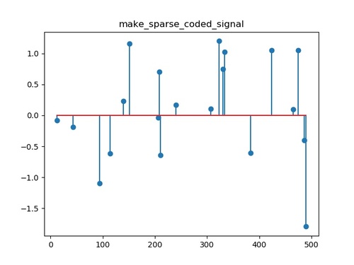
make_sparse_coded_signal()

辞書要素のスパースな組み合わせとして信号を生成します。

• 用途：分解アルゴリズム
• ドキュメント：sklearn.datasets.make_sparse_coded_signal

以下にmake_sparse_coded_signal()の使用例を示します。

from sklearn.datasets import make_sparse_coded_signal
import matplotlib.pyplot as plt

if __name__ == "__main__":

    n_samples = 1         # データ件数
    n_components = 500    # 辞書内のコンポーネントの数
    n_features = 100      # データ次元数
    n_nonzero_coefs = 20  # 各データの非ゼロ係数の数
    random_state = 1      # 乱数生成用のシード

    # make_sparse_coded_signal()を用いてデータを生成する
    data, dictionary, code = make_sparse_coded_signal(n_samples=n_samples, n_components=n_components, n_features=n_features, n_nonzero_coefs=n_nonzero_coefs, random_state=random_state)

    # 生成されたデータをプロットする
    idx = code.nonzero()
    plt.stem(idx[0], code[idx])
    plt.title('make_sparse_coded_signal')
    plt.show()

このプログラムを実行すると以下の出力結果が得られます。

make_spd_matrix()

ランダムな対称正定行列を生成します。

• 用途：分解アルゴリズム
• ドキュメント：sklearn.datasets.make_spd_matrix

以下にmake_spd_matrix()の使用例を示します。

from sklearn.datasets import make_spd_matrix

if __name__ == "__main__":

    n_dim = 5         # 行列の次元数
    random_state = 1  # 乱数生成用のシード

    # make_spd_matrix()を用いてデータを生成する
    x = make_spd_matrix(n_dim=n_dim, random_state=random_state)

    # 生成されたデータを表示する
    print('x.shape : {}'.format(x.shape))
    print(x)

このプログラムを実行すると以下の出力結果が得られます。

x.shape : (5, 5)
[[ 1.40210457 -0.94459272 -0.75472802 -1.1710128   0.39615045]
 [-0.94459272  1.58411951  0.95268323  1.67406026 -0.0559904 ]
 [-0.75472802  0.95268323  0.79047245  1.17580375 -0.11674895]
 [-1.1710128   1.67406026  1.17580375  3.04339404 -0.24525879]
 [ 0.39615045 -0.0559904  -0.11674895 -0.24525879  0.24658801]]

make_sparse_spd_matrix()

スパース対称定正行列を生成します。

• 用途：分解アルゴリズム
• ドキュメント：sklearn.datasets.make_sparse_spd_matrix

以下にmake_sparse_spd_matrix()の使用例を示します。

from sklearn.datasets import make_sparse_spd_matrix

if __name__ == "__main__":

    dim = 5              # 行列サイズ
    alpha = 0.95         # 係数がゼロである確率
    norm_diag = False    # 行列を正規化しない
    smallest_coef = 0.1  # 最小係数の値
    largest_coef = 0.9   # 最大係数の値
    random_state = 1     # 乱数生成用のシード

    # make_sparse_spd_matrix()を用いてデータを生成する
    x = make_sparse_spd_matrix(dim=dim, alpha=alpha, norm_diag=norm_diag, smallest_coef=smallest_coef, largest_coef=largest_coef, random_state=random_state)

    # 生成されたデータを表示する
    print('x.shape : {}'.format(x.shape))
    print(x)

このプログラムを実行すると以下の出力結果が得られます。

x.shape : (5, 5)
[[ 1.          0.          0.          0.          0.        ]
 [ 0.          1.          0.          0.          0.        ]
 [ 0.          0.          1.         -0.81568533  0.        ]
 [ 0.          0.         -0.81568533  1.66534256  0.        ]
 [ 0.          0.          0.          0.          1.        ]]